Introduction
Google Sheets is a popular cloud-based spreadsheet application that allows users to organize and analyze data easily. With its user-friendly interface and various functions, Google Sheets has become a valuable tool for individuals and businesses alike. One of the most commonly used functions in Google Sheets is the SUM function, which allows users to quickly add up numbers in a given range.
What is Google Sheets?
Google Sheets is a web-based spreadsheet application created by Google as part of their Google Drive suite of productivity tools. It provides users with a platform to create and edit spreadsheets, analyze data, and collaborate with others in real-time. Google Sheets is accessible via any web browser and can be used on both desktop and mobile devices.
What is the SUM Function?
The SUM function is a built-in function in Google Sheets that allows users to add up numbers in a given range or array. It is a convenient way to quickly calculate totals, averages, and other calculations that involve adding up numbers.
To use the SUM function in Google Sheets, users need to select a cell to display the sum of the values. They can then type in the formula =SUM( and select the cells or range of cells they wish to sum up. This can also be done by selecting the SUM function from the Insert tab and choosing the range of cells.
Using the SUM function in Google Sheets has several benefits. It ensures accuracy in calculations, saves time by automating the process of adding up numbers, provides for dynamic calculations in real-time, and promotes collaboration among team members by allowing multiple users to work on the same spreadsheet simultaneously.
Therefore, the SUM function in Google Sheets is a powerful tool that can simplify the process of adding up numbers and calculating totals in a spreadsheet environment. It is a feature that is easy to use and provides various benefits to users, including accuracy, efficiency, and collaboration. Whether it is for personal or professional use, the SUM function in Google Sheets can help users to streamline their work and achieve their goals.
Entering Data into Google Sheets
Google Sheets is an effective tool for organizing your data. Whether you are creating a budget, keeping track of your expenses, or creating a project report, Sheets makes it easy to do it all. However, one of the crucial things to know when using Sheets is how to enter data accurately. Here’s how to:
Entering data into Sheets
Before you can add up numbers in Sheets, you must first enter the data you want to work with. To add data to a cell:
1. Start by clicking or tapping the cell where you want to enter the information
2. Tap “Enter text or formula” to display the keyboard
3. Enter the value or text in the cell
4. Tap “Enter” to save the data
Selecting a range of cells
Once you have entered the data, you can now start the process of adding it to your spreadsheet. To do this, select the range of cells that you want to add together. You can do this by following these steps:
1. Click and drag your cursor to select the range of cells that you want to add together
2. Alternatively, you can hold down the “Shift” key and click on the cells you want to select
3. Once you have selected the cells, you are now ready to add them up using the SUM function.
Using the SUM function
Now that you have selected the range of cells that you want to add up, it’s time to use the SUM function. Here’s how to:
1. Click on the cell where you want to display the result
2. Tap “Enter text or formula” and type “=sum(“
3. Now select the cells you want to add together
4. Close the formula with “)”
5. Press “Enter” to get the result.
Therefore, knowing how to enter data into Google Sheets accurately is an essential skill that can save you time and prevent errors in your calculations. By using the SUM function, you can easily add up the numbers in your spreadsheet without having to do the math manually. Happy calculating!
Using the SUM Function
Basic formula usage for SUM function
The SUM function in Google Sheets is a powerful tool in quickly adding up numbers in a range. The basic formula for using the SUM function is to select the cell where you want to display the total and use the formula “=sum(range)” where “range” is the selection of cells to be added. This simple formula can add up any series of numbers in a selection and provide the total in a single cell.
For example, if you have a range of cells A1 to A10 that contains sales data, you can use the formula “=sum(A1:A10)” to add up all the sales values and get the total in a single cell instantly. The SUM function also provides a convenient way to check your work as it updates the total whenever the data in any of the cells in the range is changed.
Different methods of using SUM()
In addition to the basic formula usage, there are multiple methods of using the SUM function in Google Sheets based on the type and format of the data in the cells ranging from the traditional selection of cells to a more advanced array formula.
One alternative method of using the SUM function is to select a non-contiguous range of cells, such as a sum of sales in January and March but not February. To do this, select the first range using the formula “=sum(range1)+sum(range2)-sum(excluded range)”. This method only requires a few extra steps, but the outcome will be the same total.
Another way to use the SUM function in Google Sheets is by utilizing the “range1:range2” syntax, which allows you to select contiguous ranges. Using this method, you can select ranges that are diagonal on the sheet, such as D2:F4.
Lastly, you can use an array formula, which returns a range of cells instead of a single value. This formula utilizes curly braces “{}” to force the formula to calculate using all cells in the range. An example of this formula usage is “=sum({range1; range2; range3})” which would add up all the numbers in the three ranges listed.
Therefore, the SUM function in Google Sheets is an essential tool for anyone who regularly works with spreadsheets that require adding up numbers. Utilizing this function can help decrease the margin of errors from manual calculations, increase accuracy and efficiency, and provide significant time-saving benefits. By using the various methods discussed, it is possible to maximize the use of the SUM function and the overall productivity of the Google Sheets software.
Summing a Range of Cells
Google Sheets is a great way to organize and analyze data, but often we need to add up values from multiple cells. Thankfully, Sheets features a function called SUM that makes this task a breeze. Here’s a guide on how to use it effectively.
Using the SUM Function for Multiple Cells
To get started with the SUM function, first select the cell where you want to display the sum of multiple cells. Then, type in “=SUM(” followed by a range of cells you want to add up. For instance, if you want to add up cells A1 through A5, you would type in “=SUM(A1:A5)”. You can also include separate cell ranges by separating them with a comma. For example, “=SUM(A1:A5, B1:B5)” would add up the values in both ranges.
Including or Excluding Cells in the Sum
You can also choose to exclude certain cells from the sum calculation by using the minus sign. For example, “=SUM(A1:A5-B3)” would sum up cells A1 through A5 but exclude the value of cell B3. On the other hand, you can include additional cells in the sum calculation by using the plus sign. For example, “=SUM(A1:A5+B3)” would sum up all of the values in cells A1 through A5 and include the value of cell B3.
In addition, you can automate the SUM function by using it with the AutoSum feature. To use AutoSum, select the cell where you want the sum to appear and click on the AutoSum icon (Σ) in the toolbar. Sheets will automatically select the range of cells for you based on the location of your cursor.
Examples
Let’s say you have a spreadsheet with three rows containing numbers. You want to add up all the numbers in each row. Here are the steps you can follow to use the SUM function for each row:
1. Select the cell where you want the sum for the first row to appear
2. Type in “=SUM(A1:C1)” to add up all the values in the first row
3. Press “Enter” to display the result
4. Repeat steps 1-3 for the other two rows
You can also use the SUM function to add up columns or even entire sheets of data. Simply select the range of cells you want to add up and use the formula =SUM(range).
Therefore, Google Sheets’ SUM function is a simple yet powerful tool for adding up values in a spreadsheet. It can help you save time and reduce errors in your calculations. By following the steps outlined in this guide, you can easily sum up ranges of cells, include or exclude certain cells, and use AutoSum to automate the process even further.
Customizing Your SUM Function
Google Sheets’ SUM function is a powerful tool for adding up values in a spreadsheet, but it can also be customized to fit your specific needs. Here are some tips on how to further customize your SUM function.
Rounding numbers using the ROUND function
Sometimes you may want to round the sum of your values to a certain number of digits. For example, if you’re calculating money amounts, you may want to round to two decimal places. In this case, you can use the ROUND function to achieve this.
To use the ROUND function in conjunction with the SUM function, first select the cell where you want the rounded sum to appear. Then, type in “=ROUND(SUM(” followed by a range of cells you want to add up. For example, “=ROUND(SUM(A1:A5),2)” would add up cells A1 through A5 and round the result to two decimal places.
Combining the SUM and ROUND functions
Another way to customize your SUM function is to combine it with other functions, such as ROUNDUP or ROUNDDOWN. For example, if you want to round up the sum of your values to the nearest integer, you can use the SUM and ROUNDUP functions together.
To do this, first select the cell where you want the rounded-up sum to appear. Then, type in “=ROUNDUP(SUM(” followed by a range of cells you want to add up. For example, “=ROUNDUP(SUM(A1:A5))” would add up cells A1 through A5 and round the result up to the nearest integer.
By customizing the SUM function with additional functions, you can tailor it to suit your specific needs and make your calculations more accurate and efficient.
Using Conditional Summing with SUMIF
When working with large sets of data in Google Sheets, it’s often important to add up specific cells of data that meet certain conditions. This is where the SUMIF function in Google Sheets can come in handy. By using the SUMIF function, you can easily sum up data that fits your stated criteria such as a name category or dollar value within a data set.
How to sum by a single criterion
To use the SUMIF function to sum up values in Google Sheets that meet a single criterion, follow these steps:
1. Start by opening your Google Sheets spreadsheet.
2. Select the cell where you want the sum to appear.
3. Type in the SUMIF formula in the cell “=SUMIF(range, criterion, [sum_range])”.
4. Replace the “range” parameter with the series of cells you want to evaluate based on your criteria.
5. Insert your “criterion” parameter inside quotation marks. This defines what criteria your data should meet for the cell to be added up.
6. If you’re adding up a range of cells, you can include the “sum_range” parameter. This will specify the range of cells that you want to have added up.
7. Press enter and see the result.
How to sum by multiple criteria
To use the SUMIF function in Google Sheets to add up values that meet multiple criteria, follow these steps:
1. Set up your spreadsheet with the multiple criteria in separate columns, such as name and category or date and value.
2. Select the cell where you want the sum to appear.
3. Type in the SUMIFS formula in the cell “=SUMIFS(sum_range, criteria_range1, criterion1, criteria_range2, criterion2…)”.
4. Replace “sum_range” with the range of cells to be added.
5. Insert each “criteria_range” and “criterion” pair consecutively. This means, for example, criteria_range1 would be the cells where your first criterion is found, criterion1 would be the first criterion itself, criteria_range2 would be the cells where your second criterion is found, etc.
6. Press enter and see the result.
Using the SUMIF function in Google Sheets is a quick and easy way to sum up specific cells of data that meet certain conditions. By following the above steps, you can be sure to have your data accurately and quickly summarized.
Using SUMSQ
The SUMSQ function in Google Sheets is a powerful tool for calculating the sum of squares for a given sample. This function allows users to easily calculate the sum of the squares of a range of values or cells. It uses the following basic syntax:
= SUMSQ (value1, value2, value3, …)
To calculate the sum of squares, the function uses the formula:
Sum of squares = Σxi
where Σ is a fancy symbol that means the sum of the values in the range, and xi is the i-th data value.
Calculating the sum of the squares of a range
To use the SUMSQ function, simply input the range of cells containing the data you wish to calculate the sum of squares for, into the formula. For example, if you have a dataset in cells A2 to A13, you can input the following formula into any cell:
= SUMSQ (A2:A13)
This formula will return the sum of squares for the dataset.
Examples of practical use
The SUMSQ function in Google Sheets is useful for a variety of applications. For example, it can be used to calculate the variance of a sample, which is an important statistical measure used in data analysis. To find the variance of a data sample, simply use the following formula:
Variance = (1/n) * SUMSQ (xi – x̄)
where n is the number of data values, xi is the i-th data value, and x̄ is the mean of the data sample.
Another practical application of the SUMSQ function is in regression analysis, where it is used to calculate the sum of squares of errors. This is done by comparing the predicted values to the actual values, and calculating the difference between them.
Overall, the SUMSQ function in Google Sheets is a powerful tool for calculating the sum of squares for a given sample. Its simplicity and ease of use make it a valuable tool for statistical analysis and data processing.
Therefore, anyone working with large sets of data in Google Sheets should be familiar with the SUMSQ function and its many practical applications. By using this function, users can easily calculate the sum of squares of a range of values or cells, and use this information for detailed statistical analysis and data processing.
Using SERIESSUM
Understanding the function
When working with large sets of data, the SERIESSUM function in Google Sheets can be a useful tool for saving time and reducing the risk of errors. While using the SERIESSUM function may seem intimidating at first, it’s fairly straightforward. To use it, you first need to select the cell where you want the result to appear and then type in the function “=Seriessum( )” followed by the relevant parameters of the function. Additionally, the SERIESSUM function can be combined with other functions, such as the SUM function, to create more complex calculations.
Examples of practical use
Let’s take a look at some examples of SERIESSUM formulas in action. For instance, the SUM function can be used to quickly add up a list of numbers, while the SUMPRODUCT function can be used to calculate the sum of the product of two or more arrays. By mastering the SERIESSUM function, you can apply it to a wide range of financial and mathematical calculations in Google Sheets.
Using Conditional Summing with SUMIF
How to sum by a single criterion
Conditional summing is another powerful function within Google Sheets, allowing users to sum up specific cells of data that meet certain conditions. To use the SUMIF function to sum up values in Google Sheets that meet a single criterion, you need to first open your Google Sheets spreadsheet and then follow a few simple steps:
1. Select the cell where you want the sum to appear.
2. Type in the SUMIF formula in the cell “=SUMIF(range, criterion, [sum_range])”.
3. Replace the “range” parameter with the cell range you want to evaluate based on your criteria.
4. Insert your “criterion” parameter inside quotation marks. This defines what criteria your data should meet for the cell to be added up.
5. If you’re adding up a range of cells, you can include the “sum_range” parameter. This specifies the range of cells that you want to have added up.
6. Press enter and see the result.
How to sum by multiple criteria
To use the SUMIF function in Google Sheets to add up values that meet multiple criteria, follow these steps:
1. Set up your spreadsheet with the multiple criteria in separate columns, such as name and category, or date and value.
2. Select the cell where you want the sum to appear.
3. Type in the SUMIFS formula in the cell “=SUMIFS(sum_range, criteria_range1, criterion1, criteria_range2, criterion2…)”.
4. Replace “sum_range” with the range of cells to be added.
5. Insert each “criteria_range” and “criterion” pair consecutively. This means, for example, criteria_range1 would be the cells where your first criterion is found, criterion1 would be the first criterion itself, criteria_range2 would be the cells where your second criterion is found, and so on.
6. Press enter and see the result.
Using the SUMIF function in Google Sheets is a straightforward way to sum up specific cells of data that meet certain conditions. By following these steps, you can be confident that your data is accurately and quickly summarized.
Conclusion and Frequently Asked Questions
Pros and Cons of using the SUM Function
Using the SUM function in Google Sheets has many advantages, such as saving time, reducing errors, and simplifying calculations. It allows users to quickly add up a list of numbers or select a range of cells to add up, making it especially useful when dealing with large datasets. The flexibility of the formula also allows it to be combined with other functions to create more complex calculations. However, one potential drawback of using this function is that it may not be suitable for all types of data or calculations. Additionally, it is important to ensure that all cells included in the formula contain the correct data or values to avoid any miscalculations.
Frequently Asked Questions
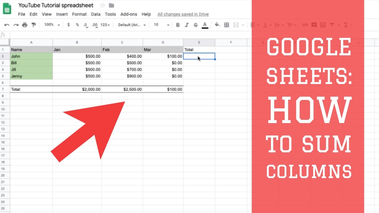
1. How do I sum a column in Google Sheets using the SUM function?
To sum a column in Google Sheets using the SUM function, simply select the cell where you want the result to appear and type in the function “=SUM(range)” followed by the cell range you want to add up. This will calculate the total of the cells in the selected range.
2. Can the SUM function be used with conditional criteria?
Yes, the SUMIF and SUMIFS functions can be used in Google Sheets to add up specific cells of data that meet certain conditions. The SUMIF function allows users to sum up values in Google Sheets that meet a single criterion, while the SUMIFS function can be used to add up values that meet multiple criteria.
3. What are the benefits of using the SUM function in Google Sheets?
Some benefits of using the SUM function in Google Sheets include saving time, reducing errors, simplifying calculations, and allowing users to add up multiple cells or select a range of cells to add up. The formula’s flexibility also allows it to be combined with other functions to create more complex calculations.
4. What potential drawbacks should be considered when using the SUM function?
One potential drawback of using this function is that it may not be suitable for all types of data or calculations. It is also important to ensure that all cells included in the formula contain the correct data or values to avoid any miscalculations.